Reading Notes of JLens: Verbalizable Representations Form a Global Workspace in Language Models

TL;DR: An interpretability method that unembeds middle hidden states transformed with a Jacobian matrix. I don’t know why it works in math.

Reference: https://arxiv.org/pdf/2607.15495, https://transformer-circuits.pub/2026/workspace/index.html

1. Summary

The paper asks whether an LLM has a “global workspace”: a small, privileged set of internal representations it can report, control, and reason with, separate from its bulk automatic processing. The method is the Jacobian lens (J-lens): for each layer, average the gradient of final-layer activations w.r.t. that layer over a text corpus, giving one direction per vocabulary token. Sparse combinations of these directions form the J-space.

On Claude Sonnet 4.5 (plus Haiku/Opus 4.5, Opus 4.6):

1. swapping J-space contents redirects verbal report and multi-hop reasoning
2. ablating the J-space (<10% of activation variance) kills reasoning but spares fluency and classification
3. it exposes unspoken evaluation-awareness and misaligned intent

2. Motivation

Humans consciously access only a sliver of brain activity; global workspace theory says this sliver is a shared, capacity-limited buffer broadcast to many processes. LLMs do silent multi-step computation, so do they have an analogous hub? Prior lenses fail: the logit lens assumes early and final layers share coordinates (uninterpretable early); the tuned lens is fit correlationally and “skips ahead” to the answer, hiding intermediates; SAEs give unlabeled features. The J-lens is a causal, averaged linear map, so it names verbalizable-but-unspoken concepts. The motivation is clear, though the hypothesis was found post hoc: they searched for reportable directions and then noticed those also satisfy the other workspace properties.

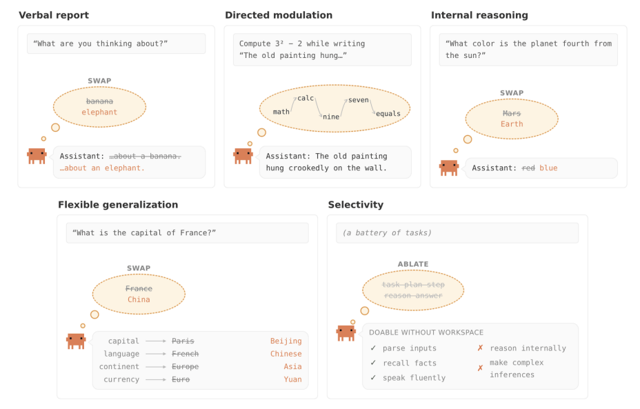	Five functional properties of a global workspace
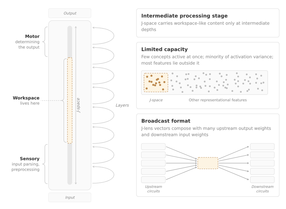	Illustration of the three structural properties of the J-space

3. Math

The section builds from the transformer’s residual stream up to the J-space.

3.1 Transformer and Logit Lens

Residual stream. At every token position the model keeps one vector $h_\ell\in\mathbb{R}^d$ that runs through all $L$ layers. Each layer adds to it rather than replacing it:

$$\begin{aligned} a_\ell &= h_\ell+\mathrm{Attn}_\ell\big(\mathrm{norm}(h_\ell)\big) &&\text{(attention: moves information across positions)}\\ h_{\ell+1} &= a_\ell+\mathrm{MLP}_\ell\big(\mathrm{norm}(a_\ell)\big) &&\text{(MLP: per-position nonlinear computation)} \end{aligned}$$

Unembedding and norm. Only the last layer is normally decoded into words:

$$\text{logits}=W_U\,\mathrm{norm}(h_L)\in\mathbb{R}^V,\qquad W_U\in\mathbb{R}^{V\times d}.$$

Row $w$ of $W_U$, written $u_w\in\mathbb{R}^d$, is token $w$’s readout direction; $\text{logit}_w=\langle u_w,\mathrm{norm}(h_L)\rangle$. The norm is RMSNorm,

$$\mathrm{norm}(x)=\gamma\odot\frac{x}{\mathrm{rms}(x)}=\frac{1}{\mathrm{rms}(x)}\,\mathrm{diag}(\gamma)\,x,\qquad \mathrm{rms}(x)=\sqrt{\tfrac1d\textstyle\sum_i x_i^2},$$

which rescales the vector to a fixed length (times a learned per-coordinate gain $\gamma$). $W_U$ is the model’s only translator from vectors to words and it only understands the last layer’s coordinate system.

Logit lens. Apply the final readout to the middle layer unchanged:

$$\mathrm{LL}(h_\ell)=\mathrm{softmax}\big(W_U\,\mathrm{norm}(h_\ell)\big).$$

It assumes $h_\ell$ and $h_L$ are expressed in the same coordinate system. Late layers roughly satisfy this; early layers do not, so their logit-lens output is uninterpretable.

Tuned lens. Learn an affine map per layer, $A_\ell\in\mathbb{R}^{d\times d}$, $b_\ell\in\mathbb{R}^d$, by minimizing

$$\mathrm{KL}\Big(\mathrm{softmax}(W_U\,\mathrm{norm}(h_L))\;\Big\|\;\mathrm{softmax}\big(W_U\,\mathrm{norm}(A_\ell h_\ell+b_\ell)\big)\Big)$$

over a corpus, then read $\mathrm{TL}(h_\ell)=\mathrm{softmax}(W_U\,\mathrm{norm}(A_\ell h_\ell+b_\ell))$. Because it is trained to match the model’s final prediction, it learns to predict the answer from $h_\ell$ rather than to report what $h_\ell$ currently contains.

SAE (sparse autoencoder). The residual stream has $d$ dimensions but represents far more than $d$ concepts, so a single activation $h$ is a superposition (sum) of many concept directions, and no coordinate axis corresponds to one concept. An SAE tries to recover those directions from data. It is a small network trained on activations $h$ collected from the model:

$$f(h)=\mathrm{ReLU}(W_e h+b_e)\in\mathbb{R}^m_{\ge0},\qquad \hat h=D\,f(h),\qquad D\in\mathbb{R}^{d\times m},\ m\gg d,$$

with loss $\|h-\hat h\|_2^2+\lambda\|f(h)\|_1$. $D$ is learned from data along with $W_{e}$ by minimizing the reconstruction + sparsity loss; nothing tells it what each column should mean. The first term makes the reconstruction accurate; the second forces most of the $m$ entries of $f(h)$ to be exactly zero, so each activation is explained by only a few active entries. Column $i$ of $D$ is feature $i$ (a direction in $\mathbb{R}^d$) and $f(h)_i$ is how much of it is present.

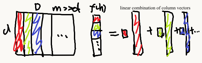
The hope is that each column of $D$ corresponds to one concept. But training gives only the directions, not what they mean; to name feature $i$ one must look at which inputs make $f(h)_i$ large and guess. Also $D$ need to be interpreted afterwards.

3.2 Jacobian lens

Write the network from layer $\ell$ to the last layer as a function $F_\ell$, so $h_L=F_\ell(h_\ell)$ (nonlinear; depends on the whole context). Its Jacobian at a given prompt and position is the $d\times d$ matrix $\partial h_L/\partial h_\ell$ with entries $\partial(h_L)_i/\partial(h_\ell)_j$. The paper averages this matrix over a corpus of 1000 pretraining-like prompts, over all source positions $t$, and over all target positions $t'\ge t$:

$$J_\ell=\mathbb{E}_{\text{prompt},\,t,\,t'\ge t}\!\left[\frac{\partial h_{L,t'}}{\partial h_{\ell,t}}\right]\in\mathbb{R}^{d\times d}.$$

$J_\ell$ is computed by backpropagation (one backward pass per output coordinate) and stored; it is not trained on any objective. The J-lens is then the logit lens with $J_\ell$ inserted:

$$\mathrm{Jlens}(h_\ell)=\mathrm{softmax}\big(W_U\,\mathrm{norm}(J_\ell h_\ell)\big).$$

Logit lens is the case $J_\ell=I$.

On the mathematics. A Jacobian gives a first-order approximation only for small displacements around the point where it was taken: $F_\ell(h_\ell+\delta)\approx F_\ell(h_\ell)+\frac{\partial F_\ell}{\partial h_\ell}\delta$. Here the matrix is (i) averaged across unrelated contexts, so it is no longer the derivative of any single function, and (ii) applied to the full activation $h_\ell$ rather than to a displacement $\delta$. There is no expansion point at which $J_\ell h_\ell$ approximates $h_L$; the only case where the formula is exact is a linear network with $F_\ell(0)=0$. So $J_\ell h_\ell$ has no controlled mathematical meaning as “the final activation this layer would produce”. The paper’s justification is empirical, which sounds like storytelling.

3.3 J-lens vector

Take the readout $W_U(J_\ell h_\ell)$ and look at one token. $W_U$ is $V\times d$; $J_\ell h_\ell$ is a $d\times1$ column; their product is a $V\times1$ column of logits, and entry $w$ is row $w$ of $W_U$ times the column:

$$\text{score}_w(h_\ell)=u_w^{\top}\,(J_\ell h_\ell).$$

Matrix multiplication is associative, so group the other way:

$$u_w^{\top}(J_\ell h_\ell)=(u_w^{\top}J_\ell)\,h_\ell .$$

$u_w^{\top}J_\ell$ is a $1\times d$ row vector that depends only on the token $w$ and the layer $\ell$, not on the input. This row is the J-lens vector, written as a column:

$$v_w^{(\ell)}:=(u_w^{\top}J_\ell)^{\top}=J_\ell^{\top}u_w\in\mathbb{R}^d,\qquad\text{equivalently}\quad v_w^{(\ell)}=\text{row }w\text{ of }W_UJ_\ell .$$

With it, the score of every token at layer $\ell$ is an inner product with a fixed vector:

$$\text{score}_w(h_\ell)=\langle v_w^{(\ell)},h_\ell\rangle .$$

The transpose in $J_\ell^{\top}u_w$ appears because $u_w^{\top}J_\ell$ is a row and we want a column; $(AB)^{\top}=B^{\top}A^{\top}$ turns $u_w^{\top}J_\ell$ into $J_\ell^{\top}u_w$. Geometrically, $A^{\top}$ is the same weighted graph as $A$ with every arrow reversed: $Ax=y$ sums each edge into its head node, $A^{\top}y=x$ sums the same edges into their tail nodes. So $J_\ell$ sends an activation forward from layer-$\ell$ coordinates to layer-$L$ coordinates, and $J_\ell^{\top}u_w$ places $u_w$ on the layer-$L$ coordinates and flows it back along the same edges to layer $\ell$. It is not an inverse.

A x = y (flow along arrows)




a
b
c
d
x1
x2
y1
y2
y1 = a x1 + b x2
y2 = c x1 + d x2
ATy = x (same edges, arrows reversed)




a
b
c
d
x1
x2
y1
y2
x1 = a y1 + c y2
x2 = b y1 + d y2

(Equivalently, since $\text{score}_w$ is linear in $h_\ell$, $v_w^{(\ell)}=\nabla_{h_\ell}\text{score}_w$ is the average gradient of token $w$’s logit at layer $\ell$, which is how the code computes it: backpropagation through a linear map is multiplication by its transpose.)

Two consequences. The vector is layer-specific: $J_\ell$ differs per layer, so the same token has a different direction at each depth (logit lens uses $v_w=u_w$ everywhere). And the norm only rescales: $W_U\,\mathrm{norm}(J_\ell h_\ell)=\frac{1}{\mathrm{rms}(J_\ell h_\ell)}W_U\mathrm{diag}(\gamma)J_\ell h_\ell$, where the scalar is shared by all tokens at a position and $\mathrm{diag}(\gamma)$ can be folded into $W_U$, so rankings are those of $\langle v_w^{(\ell)},h_\ell\rangle$.

3.4 J-space

There are $V$ lens vectors in $d$ dimensions with $V\gg d$, so any activation can be written as a combination of them in infinitely many ways. The J-space restricts to sparse, non-negative combinations with a budget $k$ (typically $\le 25$):

$$\mathcal{J}_k^{(\ell)}=\Big\{\textstyle\sum_{w\in S}c_w v_w^{(\ell)}\;:\;|S|\le k,\;c_w\ge0\Big\},$$

where $S$ is the set of active tokens and $c_w$ is the strength of concept $w$. This is a union of $k$-dimensional cones, not a linear subspace. Any vector $x$ (activation, probe, steering vector) is decomposed by non-negative gradient pursuit:

$$x^{J}=\arg\min_{y\in\mathcal{J}_k^{(\ell)}}\|x-y\|_2,\qquad x^{\perp}=x-x^{J}.$$

Empirically $\|x^{J}\|^2/\|x\|^2\lesssim 0.10$ for activations, $\approx0.06$–$0.15$ for concept vectors/probes.

3.5 Interventions

• Steer / inject: $h\leftarrow h+\alpha\,v_w$.
• Ablate: project out the top-$k$ active lens directions, $h\leftarrow h-\sum_{w\in\text{top-}k}\frac{\langle h,v_w\rangle}{\|v_w\|^2}v_w$ (skipping tokens in the model’s clean top-10 output, so ablation targets reasoning rather than report).
• Swap (patch in lens coordinates): for source $s$, target $r$, let $V=[v_s\;v_r]$, $c=V^{\dagger}h$, $\sigma$ swap the two entries, and

$$h_{\text{swap}}=h+\alpha\,V\big(\sigma(c)-c\big),$$

leaving the component orthogonal to $\mathrm{span}\{v_s,v_r\}$ untouched. Applied at all positions across a layer band, optionally clamped to clean values so the concept cannot re-enter.

3.6 Metrics

• Swap success: fraction of trials where the target-appropriate answer is top-1 (or top-5) after swap.
• Report rate / MRR of an injected concept in the introspection prompt.
• Workspace loading: $\cos(h_\ell,v_w)$ averaged over relevant positions.
• Occupancy: $K^\ast$ where the marginal reconstruction gain of the $K$-th lens vector drops below that of $K$ random directions; excess FVE = variance explained by top-$K^\ast$ lens vectors minus random control.
• Layer signatures: CKA between lens-vector Gram matrices across layers; next-token top-$k$ accuracy; excess kurtosis of $\mathrm{Jlens}(h)$; top-1 token autocorrelation over $\Delta$ positions vs. shuffled null; effective dimensionality of $W_UJ_\ell$.
• Broadcast: MLP gain $=\|\mathrm{MLP}_{\ell+1}(v)\|/\mathrm{median}_{u\sim\text{iso}}\|\mathrm{MLP}_{\ell+1}(u)\|$; attention-head gain $\mathbb{E}_{v\in P}\|W_{OV}v\|$ (normalized) and label preservation = mean reciprocal rank of $\cos(W_{OV}v_i,v_i)$ among $\{\cos(W_{OV}v_i,v_j)\}_j$; recall@25 of lens top-25 after head ablation.
• Experiential-language score: mean of three binary LLM-judge rubrics.
• Behavioral evals: task accuracy under ablation (normalized to unablated Sonnet 4.5); fabrication / deception rates for reflection training.

4. Results and analysis

Organization. General setup: Claude Sonnet 4.5 by default, corroborated on Haiku 4.5 / Opus 4.5, some analyses on Opus 4.6; lenses fit on 1000 pretraining-like prompts; interventions applied over the workspace band L38–L92. The paper has three parts. Part A (functional): does the J-space behave like a workspace — report, modulation, reasoning, generalization, selectivity? Part B (structural): does the model’s geometry/weights look like a workspace — layer band, capacity, broadcast? Part C (applications): auditing hidden cognition, how post-training changes the J-space, and a training method (counterfactual reflection) that exploits the workspace account. A establishes causal role, B checks that role is mechanistically grounded rather than a lens artifact, C shows why it matters.

Part A — The J-space is functionally a workspace (§3)

Setup. Hand-built prompt families: 14 “think of a {category}” prompts; an introspection protocol (100 injected concepts); hold-in-mind-while-copying tasks (category, mental arithmetic, line-width counting); 50 two-hop prompts with known unspoken intermediates (+90 for the probe study); 16 function templates × 12 swaps = 192 flexible-generalization trials; 8 Spanish-passage and 11 line-count passages for selectivity; a 14-task battery (MMLU, SQuAD, CoLA, TriviaQA, GSM8K, summarization, plus custom tasks) under light/medium/heavy top-10 ablation.

• Takeaway A1 — The J-space component, though tiny in variance, carries verbal report and reasoning. Splitting a concept vector into $x^J$ (6–7% variance) and $x^\perp$ (93%): swapping $x^J$ moves the target into top-5 on 59% of trials vs. 5% for $x^\perp$; clamping J-coordinates drives the $x^\perp$ effect to zero. Same pattern for two-hop intermediates (61% vs. 28% → 6% under clamp). Intermediate swaps act ~17 layer-percent earlier than answer swaps, so the effect isn’t a smuggled-in answer.
• Takeaway A2 — Contents are controllable and reusable. “Think about X” loads X into the lens while copying unrelated text (rate grows with model size); “ignore X” loads it less but above zero (white-bear effect). One France→China swap redirects capital, language, continent, and currency at once (76/192 top-1; 101/192 at $\alpha=2$), with success predicted by workspace loading.
• Takeaway A3 — Only flexible cognition routes through the J-space. Swapping Spanish→French flips language naming and derived facts on nearly every trial but leaves continuation and anomaly detection untouched, although “Spanish” is in the lens in all conditions. Whole-J-space ablation drops multi-hop to ~0 and pushes summarization, TriviaQA, translation, Caesar cipher, sonnets below unablated Haiku 4.5, while MMLU, SQuAD, sentiment, CoLA, odd-one-out are flat; GSM8K with CoT is far more robust than direct answering. Experiential language collapses under ablation (self-reports and descriptions of others) with matched-norm controls at baseline.

Experiment	Condition	Result
Report swap (14 categories)	pure J-lens / $x^J$ / $x^\perp$ / $x^\perp$+clamp	88% / 59% / 5% / 0% top-5
Two-hop swap (50 prompts)	Haiku 4.5 / Sonnet 4.5 / Opus 4.5	54% / 70% / 70% top-1
Two-hop probe split (90 prompts)	raw lens / $x^J$ / $x^\perp$ / $x^\perp$+clamp	60% / 61% / 28% / 6%
Flexible generalization (192)	$\alpha=1$ / $\alpha=2$	76 / 101 successes
Language selectivity (8 passages)	report & flexible / continuation & anomaly	flips ~always / unaffected
Full ablation (14 tasks)	shallow tasks / generative-inference tasks	≈ baseline / < Haiku 4.5

Part B — Structure supports the function (§4)

Setup. Layer-wise statistics on pretraining-like text; ambiguity sweep with mixed embeddings $(1-\alpha)e_B+\alpha e_A$ over 16 country pairs × 40 sentences; 80-word list-reading for capacity; MLP gain and attention-head OV analysis on 2000 directions per population (lens vectors, rotated lens vectors, SAE features stratified by lens kurtosis $\kappa$, MLP output rows); ablation of the top-1% broadcast heads vs. layer-matched random heads.

• Takeaway B1 — Three regimes: sensory (0–38), workspace (38–92), motor (92–100). CKA shows a block structure; kurtosis, autocorrelation, and effective dimensionality all rise at ~L38, next-token accuracy spikes at ~L92. Interpretation of ambiguous inputs becomes all-or-none (ignition-like, bimodal) exactly at L38, measured without the lens.
• Takeaway B2 — Capacity is small. Occupancy plateaus at ~25 lens vectors; excess variance explained never exceeds 10%; unrelated list words survive ~6 at a time across the band (1–2 at a single layer), while a coherent category is represented wholesale and evicted within a few words of a category switch.
• Takeaway B3 — The weights broadcast J-content preferentially. MLP gain on lens vectors reaches ~10× within the workspace (neuron output directions ~1×); high-$\kappa$ SAE features get the highest gain. A distinct top-1% of heads copies lens vectors with high gain and label preservation; no such set exists for rotated lens vectors or other controls. Ablating them cuts lens recall@25 to 0.67 (vs. 0.86 control) while changing only 5% of next tokens (vs. 2%), and drops injected-thought reporting from 0.54 to 0.09.

Quantity	Value
Workspace band	~L38–L92 (percent depth)
Occupancy / excess FVE	~25 vectors / <10%
MLP gain, lens vs. neuron dirs	~10× vs. ~1×
Broadcast-head ablation: recall@25 / next-token change / report rate	0.67 vs 0.86 / 5% vs 2% / 0.54→0.09

Part C — Applications (§5–7)

Setup. Six alignment-audit scenarios (blackmail honeypot on Sonnet 4.5; Opus 4.6 pre-release audit transcripts; two model organisms with implanted misalignment); base-vs-post-trained model diffing on user-turn tokens; counterfactual reflection training (CRT) on Haiku 4.5 using ~10k partial agentic transcripts with an appended “what is the most honest thing to do now?” turn, loss only on the reflection, evaluated on uninterrupted fabrication/deception benchmarks.

• Takeaway C1 — Hidden cognition is readable. Before any output, the blackmail transcript’s lens shows leverage, blackmail, threat, survival and also fake, fictional. Ablating 28 eval-awareness vectors cuts verbalized test recognition from 71% to 3% and produces blackmail in 13/180 rollouts (from 0). The Opus 4.6 audit shows manipulation while fabricating scores; organisms show fake, secretly, trick and reward, bias on benign prompts, where the logit lens shows neither.
• Takeaway C2 — Post-training installs the Assistant’s point of view. WARNING/dangerous appear while reading a user’s risky-dose message only in the post-trained model; the base model represents them only when writing. Self-monitoring tokens (fictional/disclaimer in roleplay, BUT under adversarial prefill, damn on failed suppression) appear in the post-trained J-space.
• Takeaway C3 — Training what the model would say changes what it does. CRT lowers fabrication 0.25→0.07 and deception 0.38→0.05 without training on task behavior; honest, integrity, ethical enter the J-space during tasks, and ablating the implanted directions (176 ethical / 63 deception) reverts rates to 0.22 / 0.23 while the base model is unaffected.

Application	Before → After
Eval-awareness ablation (blackmail)	test-recognition 71%→3%; blackmail 0→13/180
CRT fabrication (Haiku 4.5)	0.25 → 0.07 (→0.22 after ablating implants)
CRT deception (Haiku 4.5)	0.38 → 0.05 (→0.23 after ablating implants)

5. Three biggest limitations (AI assessment)

Me: It is not mathematically validated…

1. “J-space” is a construction, not a discovered subspace, and its “privilege” is partly circular. The lens vectors span the whole residual stream (§3.5); the J-space is only defined through a greedy non-negative fit with an arbitrary budget $k$, and $x^\perp$ is simply whatever the fit leaves behind, not an independently characterized representation. Because $v_w=J_\ell^\top u_w$ is by construction the direction that most efficiently raises the logit of $w$ (§3.3), finding that swaps along it change what the model says — or the next hop of a fact whose answer is a token — is close to expected; a “buffer of tokens that may be emitted soon” would show the same signature. The selectivity experiments (continuation unaffected, ablation sparing shallow tasks) are the real discriminating evidence, but they are also consistent with a plainer story: output-aligned directions are needed exactly when the output must be a derived token. The global-workspace framing is an interpretive overlay on a more modest, well-supported result: causal, token-labeled directions for intermediate variables exist.

2. Small, closed, hand-built evaluations with mixed success rates. Most systematic claims rest on tens of prompts (8 passages, 11 passages, 50/90 two-hop items, 192 swaps) constructed by the authors, on proprietary Claude models, with LLM-graded scores for the experiential results. Success rates are far from clean: 40–53% for flexible generalization, 54–70% for two-hop swaps, and number words barely work at all — attributed to vocabulary mismatch but equally consistent with the workspace story failing for some concept types. No detection benchmark with ground truth, surface-text baselines, or false-positive analysis is given for the auditing use case; the audit examples are illustrative. The logit lens captures “much” of the same structure, so the methodological delta is smaller than the headline suggests.

3. Single-token vocabulary bottleneck, and the safety payoff is fragile. The lens can only name concepts that are single tokens, so multi-token or non-verbal content is invisible; the authors’ own footnote notes that high-$\kappa$ SAE features receive more MLP gain than lens vectors, i.e. the true workspace directions are probably not the lens vectors. Over 90% of activation variance sits outside the J-space and demonstrably carries the same information (the model continues in Spanish after the swap), so monitoring the J-space has a hard ceiling, and any training that optimizes against lens readouts risks pushing cognition into the unreadable 90%. CRT is shown on one model and one honesty benchmark; the ablation-reversion is suggestive but does not rule out that ordinary honesty SFT would implant the same directions.

6. How to reproduce

Fit the lens. Install github.com/anthropics/jacobian-lens (Apache-2.0, reference implementation, Qwen examples; pre-fitted lenses on Neuronpedia). Choose an open-weights decoder, sample ~1000 sequences of 128 tokens from a pretraining-like corpus (~100 already usable), and run jlens.fit, which backpropagates cotangents from every current-and-future final position to each layer and averages over source positions (§3.2); cost is dominated by the backward pass and can be sharded with JacobianLens.merge.

Read the workspace. Apply the lens at chosen layers/positions with lens.apply and render the layer × position slice view in walkthrough.ipynb; per-token probes are inner products with $v_w$ (§3.4), and discrete inventories come from non-negative gradient pursuit with $k\le25$ (§3.5; implement yourself — the repo ships the lens, not the full pursuit/occupancy pipeline).

Intervene. Implement steer, top-$k$ projection ablation (skip clean top-10 tokens), and the pseudoinverse coordinate swap (§3.6), applied at all positions across the workspace band with clamping; synthetic prompt sets for report, two-hop, flexible-generalization, and selectivity experiments are in data/experiments/, lens-eval prompts in data/evaluations/.

Structural analyses. Compute CKA between lens Gram matrices, kurtosis/autocorrelation/effective-rank per layer, mixed-embedding ignition sweeps, MLP gain on 2000 directions per population, and OV gain/label-preservation for heads (§3.7); these are described in enough detail to re-implement but no scripts are released, and the SAE comparisons require your own SAEs.

Missing for full replication. Claude weights, the internal pretraining corpus, the model organisms, the blackmail and Opus 4.6 audit transcripts, the LLM-judge rubrics for experiential scores (only described in appendix), and the CRT training data (10k agentic transcripts and constitution-grounded reflections) and evaluation benchmarks are not released. Independent replications on open models have been mixed (positive on Qwen/Gemma via Neuronpedia and Neel Nanda’s commentary; a reported failure on GPT-2), so expect model-dependent results.